次轴

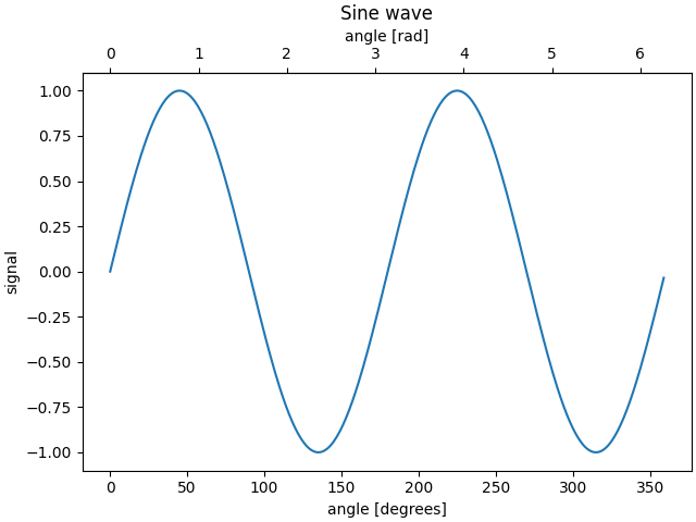
有时我们想要一个绘图上的辅助轴，例如在同一个绘图上将弧度转换为度数。我们可以通过axes.Axes.secondary_xaxis和 制作一个只有一个轴可见的子轴来做到这一点axes.Axes.secondary_yaxis。通过在函数关键字参数的元组中提供正向和反向转换函数，此辅助轴可以具有与主轴不同的比例：

import matplotlib.pyplot as plt
import numpy as np
import datetime
import matplotlib.dates as mdates
from matplotlib.ticker import AutoMinorLocator

fig, ax = plt.subplots(constrained_layout=True)
x = np.arange(0, 360, 1)
y = np.sin(2 * x * np.pi / 180)
ax.plot(x, y)
ax.set_xlabel('angle [degrees]')
ax.set_ylabel('signal')
ax.set_title('Sine wave')


def deg2rad(x):
    return x * np.pi / 180


def rad2deg(x):
    return x * 180 / np.pi


secax = ax.secondary_xaxis('top', functions=(deg2rad, rad2deg))
secax.set_xlabel('angle [rad]')
plt.show()

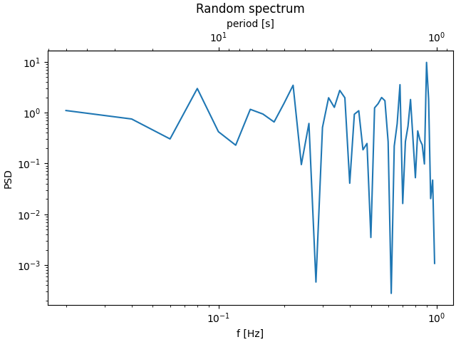
这是以对数尺度从波数转换为波长的情况。

笔记

在这种情况下，父级的 xscale 是对数的，因此子级也是对数的。

fig, ax = plt.subplots(constrained_layout=True)
x = np.arange(0.02, 1, 0.02)
np.random.seed(19680801)
y = np.random.randn(len(x)) ** 2
ax.loglog(x, y)
ax.set_xlabel('f [Hz]')
ax.set_ylabel('PSD')
ax.set_title('Random spectrum')


def one_over(x):
    """Vectorized 1/x, treating x==0 manually"""
    x = np.array(x).astype(float)
    near_zero = np.isclose(x, 0)
    x[near_zero] = np.inf
    x[~near_zero] = 1 / x[~near_zero]
    return x


# the function "1/x" is its own inverse
inverse = one_over


secax = ax.secondary_xaxis('top', functions=(one_over, inverse))
secax.set_xlabel('period [s]')
plt.show()

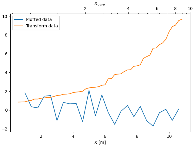
有时，我们希望将坐标轴关联到来自数据的临时转换中，并且是根据经验得出的。在这种情况下，我们可以将正向和逆变换函数设置为从一个数据集到另一个数据集的线性插值。

笔记

为了正确处理数据边距，映射函数（forward在inverse本例中）需要定义为超出标称绘图限制。

在 numpy 线性插值的特定情况下，可以通过提供可选的关键字参数left，rightnumpy.interp来任意强制执行此条件，以便将数据范围之外的值映射到绘图限制之外。

fig, ax = plt.subplots(constrained_layout=True)
xdata = np.arange(1, 11, 0.4)
ydata = np.random.randn(len(xdata))
ax.plot(xdata, ydata, label='Plotted data')

xold = np.arange(0, 11, 0.2)
# fake data set relating x coordinate to another data-derived coordinate.
# xnew must be monotonic, so we sort...
xnew = np.sort(10 * np.exp(-xold / 4) + np.random.randn(len(xold)) / 3)

ax.plot(xold[3:], xnew[3:], label='Transform data')
ax.set_xlabel('X [m]')
ax.legend()


def forward(x):
    return np.interp(x, xold, xnew)


def inverse(x):
    return np.interp(x, xnew, xold)


secax = ax.secondary_xaxis('top', functions=(forward, inverse))
secax.xaxis.set_minor_locator(AutoMinorLocator())
secax.set_xlabel('$X_{other}$')

plt.show()

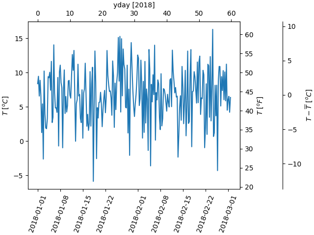
最后一个示例在 x 轴上将 np.datetime64 转换为 yearday，在 y 轴上将摄氏度转换为华氏度。请注意添加了第三个 y 轴，并且可以使用 float 作为 location 参数来放置它

dates = [datetime.datetime(2018, 1, 1) + datetime.timedelta(hours=k * 6)
         for k in range(240)]
temperature = np.random.randn(len(dates)) * 4 + 6.7
fig, ax = plt.subplots(constrained_layout=True)

ax.plot(dates, temperature)
ax.set_ylabel(r'$T\ [^oC]$')
plt.xticks(rotation=70)


def date2yday(x):
    """Convert matplotlib datenum to days since 2018-01-01."""
    y = x - mdates.date2num(datetime.datetime(2018, 1, 1))
    return y


def yday2date(x):
    """Return a matplotlib datenum for *x* days after 2018-01-01."""
    y = x + mdates.date2num(datetime.datetime(2018, 1, 1))
    return y


secax_x = ax.secondary_xaxis('top', functions=(date2yday, yday2date))
secax_x.set_xlabel('yday [2018]')


def celsius_to_fahrenheit(x):
    return x * 1.8 + 32


def fahrenheit_to_celsius(x):
    return (x - 32) / 1.8


secax_y = ax.secondary_yaxis(
    'right', functions=(celsius_to_fahrenheit, fahrenheit_to_celsius))
secax_y.set_ylabel(r'$T\ [^oF]$')


def celsius_to_anomaly(x):
    return (x - np.mean(temperature))


def anomaly_to_celsius(x):
    return (x + np.mean(temperature))


# use of a float for the position:
secax_y2 = ax.secondary_yaxis(
    1.2, functions=(celsius_to_anomaly, anomaly_to_celsius))
secax_y2.set_ylabel(r'$T - \overline{T}\ [^oC]$')


plt.show()

参考

此示例中显示了以下函数、方法、类和模块的使用：

• matplotlib.axes.Axes.secondary_xaxis

• matplotlib.axes.Axes.secondary_yaxis